Predicting the Market via Geometric Brownian Motion
Introduction:
Geometric Brownian Motion is widely used to model market behavior of financial asset prices. By utilizing historic price information, the forecasted price is based on the assumption that returns are normally distributed (or that the price is log-normally distributed). This has been popularly used on traditional financial assets, but with the rapidly increasing interest in cryptocurrencies as a new financial class, there is new territory for geometric Brownian motion to be applied.
Utilizing Monte Carlo simulations, financial risk of various assets can be assessed by generating thousands of geometric Brownian motion realizations to calculate mean prices and confidence intervals on future asset prices.
As noted above, because these applications have been popularly used to model market behavior, there are comparable metrics to measure implementation performance before attempting to model cryptocurrencies (Bitcoin).
GitHub Repository:
GitHub repo developed for this project: https://github.com/ishengy/gbm_price_forecasting
Methodology:
Standard Geometric Brownian motion assumes that the noise is normally distributed. This assumption should be checked on the available data to determine if standard geometric Brownian motion would be an acceptable method to model/forecast market prices. Stock prices are log-normally distributed, but returns (noise) follow a gaussian behavior. The returns histogram will be plotted against a normal distribution line, and a Q-Q plot will also be plotted to determine if the behavior can be described by a normal distribution.
The multiple day (step) predictions can be applied over a set period to determine how well it forecasts future values of market price. In the research paper Stock Price Predictions using a Geometric Brownian Motion paper from Uppsala University, it was determined that a training set of 60 days produced the best predictions based on the mean squared value (MSE).
Instead of re-creating the procedure described in that research paper, root mean squared error (RMSE) will replace mean squared error (MSE) because RMSE is in the same units as the dependent variable, which provides better interpretability. Additionally, because this paper will be looking across three different types of financial assets (stock options, ETFs, cryptocurrencies), the RMSE will be normalized (nRMSE) so that the values can be compared across all assets since RMSE will only make sense within the domain that it is calculated.
100,000 30-day geometric Brownian motion simulations will be generated from training sets of 30 to 100 days each, and the resulting simulations are compared to actual (test) market prices to obtain the RMSE, nRMSE, and MAPE.
Another interesting methodology that the same research paper conducts is examining the experimental probability of predicting the correct direction of the price change. According to the same research paper, 100-day sets produced the most accurate direction prediction. To perform this experiment, 100,000 one-day simulations will be generated for training sizes from 30 to 100 each. The resulting experimental prices will be subtracted by the true s(t-1) price, and the direction will be checked against the true price change direction of s(t)-s(t-1).
A two-tailed t-test with a critical value of 5% will be conducted to determine if there are any significant differences between the forecasting capabilities of the varying training set sizes to determine the best training size that balances the forecasting accuracy and directional accuracy.
When the most accurate training set(s) are determined, sample Geometric Brownian motion realizations will be generated and plotted against the actual data points.
The final method to attempt is a moving training set. Theoretically, the farther the dataset goes out, the less likely that a static training set would be representative of the current or future states, so having a training set that moves (or updates) as actual data comes in would be valuable went utilizing this model long-term. To simulate this, the forecasting length will be increased to 120 days.
Results:
AMD Stock (AMD):
Analysis of Returns:
The distribution of returns on AMD stock is normal with a couple outliers on the right end tail, but the behavior appears to be normal. Similarly, the Q-Q plot shows that the behavior can mostly be described by a normal distribution, but the points that trail off at the end indicate a bit of right skewedness.

Forecasting Predictions (Stationary Training Set):
The expected RMSE and expected MAPE for the 40-day set is the lowest amongst the training sets. This differs from the findings in research paper from Uppsala University, which concluded a 60-day training set to be the most accurate.
In comparison to the same paper’s results of the 100-day set being the most accurate training size when it comes to predicting the correct direction of the price change, the testing set on AMD stock prices results in a training size of 90 being the most accurate.

The expected RMSE of each training size are all similar; to determine if there is a statistically significant difference between each training size’s expected RMSE, a two-tailed t-test will be performed against each permutation:

The table above displays the calculate p-values of each tested permutation of training sizes. With a critical value of 5%, this test reveals that there is no statistically significant difference between 40 and 50 days, but there is a difference between the rest. Given that the 50-day training set results in a higher directional accuracy, that should be the better choice between the two.
Sample 30 Business Day Forecasts:

Forecasting Predictions (Moving Training Set):
A 120-day simulation with a stationary and non-stationary training set was conducted – the results are as follows:
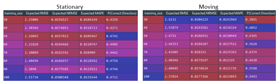

As expected, the accuracy of the stationary training set decreases as the projection length increases. The lowest RMSE is produced by a training set of size 30, but it also results in the worse accuracy for predicting directional change. The two-tailed t-tests reveal that there is no statistically significant difference between the 30- and 50-day training set, so sticking with the 50-day set actually results in better accuracy for predicting directional change; unfortunately, it’s still far below the short-term results.
On the other hand, the moving training set results in slightly higher RMSE – with a 100-day training set resulting in the lowest RMSE of 2.37, but the directional accuracy is already significantly better at 55%. The t-test reveals that there’s no significant difference between the 100-day set and any set between 50 and 90 days. Thus, a 60-day set would result in a slightly better directional accuracy of 56.2%, which is actually 5% higher than the short-term accuracy.
S&P500 ETF (SPY):
Analysis of Returns:
The distribution of returns on SPY is a bit skewed to the left. However, it does still hold a general normal shape. The Q-Q plot reinforces this assessment since only a few of the points trail off in the beginning, indicating left skewedness.

Forecasting Predictions (Stationary Training Set):
For the S&P500, the training size that resulted in the lowest RMSE and MAPE is the 50-day training set. When attempting to determine the best training size to measure direction accuracy, the size that produced the most accurate direction predictions is the 90-day set. These results are similar to the AMD results.

Running the t-tests on these sets of training data reveals that the 50-day training set’s difference is statistically significant from all other training sizes. Once again, there is going to be a compromise between RMSE and directional accuracy, but the 50-day set has a respectable accuracy of 57%, so the impact will be minimized.

However, when looking at the normalized RMSE (nRMSE), it’s approximately 2 to 2.5 times smaller than AMD’s nRMSE. This seems to be expected given that the S&P500 by definition would have less variance than a single stock option because the variance of ETFs is based on multiple uncorrelated stock options. The smaller variance would result in more predictable and consistent behavior to forecast due to the tighter bounds.
Sample 30 Business Day Forecasts:

Forecasting Predictions (Moving Training Set):
Conducting another prolonged forecasting test with stationary and moving training sets results in the following:
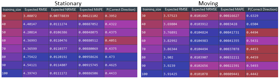

As expected, the stationary training set experienced significantly reduced directional shift accuracy. A 30-day training set surprisingly results in a better expected RMSE than the short-term results. Unfortunately, this improvement also results in the worst directional accuracy at barely 40%. The rest of the results are already worse since the short-term results has significantly lower RMSE and directional accuracies.
As for the moving training set, the expect RMSE is comparable to the short-term results, with the lowest RMSE of 3.58 being produced by a 30-day training set. The t-test reveals that training set sizes of 40 to 60 days are not significantly different. This would allow us to conclude that the 40-day training set would be the best option since it results in the highest directional accuracy of 65%, which is 8% higher than the short-term accuracy.
Bitcoin (BTC):
Analysis of Returns:
While the general shape and the Q-Q plot can be interpreted as generally normal, the normal distribution does not cover the peaks of the returns enough. Kernel density estimation can be employed to create a distribution that would capture this behavior better.

Forecasting Predictions (Stationary Training Set):
A training size of 80-days results in the best expected RMSE and MAPE. An interesting note when looking at the accuracy of directional change is that model produces one of the most accurate results amongst the three assets examined, with a 50-day training set producing an experimental probability of 63.6%. This is an unexpected result given that cryptocurrencies are more volatile than traditional financial assets, and the assumption of normality by the geometric Brownian motion seemed to be incorrect based on the returns distribution.
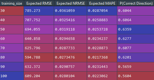
When running the t-test against the expected RMSE of each permutation, the training sizes of 60 to 100 are not statistically significant different against the 80-day set. Given that the 60-day set produces the second most accurate directional accuracy, that should be the best choice of a training set size with minimal compromises in the RMSE.

Looking at the expected nRMSE values show expected results given the volatile nature of cryptocurrencies. The expected nRMSE are slightly higher than that of AMD’s, and three times higher than that of the S&P500’s nRMSE. This means that the forecasting capabilities of standard geometric Brownian motion isn’t as accurate in comparison to its applications to traditional assets where a normal distribution assumption is more acceptable.
When attempting the same procedure with kernel density estimation (KDE) to model the change in price, the results are surprisingly very similar. Interestingly enough, the previously mentioned research paper had a similar result even when it was noted that the Cauchy distribution fit better than a normal distribution.

Sample 30 Business Day Forecasts:

Forecasting Predictions (Moving Training Set):
Conducting another prolonged forecasting test with stationary and moving training sets results in the following:


Oddly enough, the prolonged forecasting timeframe seemed to have resulted in better RMSE than the short-term predictions. Despite that improvement, the directional accuracy pales in comparison. While the 50-day training set isn’t statistically different from the 30 or 40-day results, directional accuracy barely reaches 40%.
Looking at the moving training set, we actually end up with better RMSE, and comparable directional accuracy. A 30-day training set results in an RMSE that is half of the short-term results, as well as a directional accuracy that is practically equivalent.
This behavior could once again be explained by the volatility of cryptocurrencies – high volatility would cause the training set to be less representative of the current or future state in a shorter timeframe. Thus, a moving training set that updates frequently would be better suited to combat this behavior than a stationary one.
Conclusion:
From an implementation stand point against the traditional assets, the performance matched those in the cited papers. The MAPEs for the simulated AMD stock fell within one standard deviation of the MAPE calculated against the Australian stocks. The results didn’t conclude the same effective sample size when looking for the best performance in comparison to the paper from Uppsala University, but different stocks were chosen to measure this performance, as well as different performance metrics (MSE vs RMSE). Thus, the comparison against that paper isn’t one-to-one.
In regards to directional accuracy, both papers concluded accuracies in the lower 50% range. The main abnormality between the cited papers to note is that the model performed on Australian stocks had a max accuracy of 85%. This was significantly higher than both results obtained by the paper from Uppsala University and from this research too.
When moving to measure forecasting performance on Bitcoin, the expected normalized RMSE performed slightly worse than AMD’s nRMSE, which is expected behavior due to the volatile nature of cryptocurrency. However, the directional accuracy was surprisingly accurate, with correct predictions in the upper 50% and lower 60%. These results seem surprising because Bitcoin was experiencing a bull-market in this timeframe - this phenomenon would have resulted in a left-skewed distribution that would’ve resulted in more incremental than decremental direction changes.
The concluding results from this research indicates that the Bitcoin, and other cryptocurrencies that are highly correlated (such as Ethereum), can be modeled as Geometric Brownian Motions with comparable accuracy to stock prices, but knowingly less so than ETFs.
Bibliography:
1. Lidén, J. (2018, May 28). (thesis). Stock Price Predictions using a Geometric Brownian Motion. Uppsala University. Retrieved from https://uu.diva-portal.org/smash/get/diva2:1218088/FULLTEXT01.pdf
2. Reddy, Krishna and Clinton, Vaughan, Simulating Stock Prices Using Geometric Brownian Motion: Evidence from Australian Companies, Australasian Accounting, Business and Finance Journal, 10(3), 2016, 23-47. doi:10.14453/aabfj.v10i3.3